Mean-squared error versus cross-entropy
This post is about multinomial probability distributions $p = (p_1, \ldots ,p_N)$ where $\sum_i p_i = 1$.
We often need to compare two such distributions using a ‘distance’ function $d(p,q)$. For example (and the motivation for this blog post was a recent conversation about this case), the error that gets back-propagated when we train a neural network classifier: $p$ is the one-hot vector specifying the class of a training example, and $q$ is the corresponding soft-max output of the network.
For this, one might use the good old Euclidean metric \[ d_{\rm Eucl}(p,q) = \left( \sum_i | p_i - q_i |^2 \right)^\frac{1}{2}. \]
Alternatively, one can use cross-entropy (not a metric, but motivated from information theory) \[ d_{\rm CE}(p,q) = \sum_i - p_i \log q_i . \]
Discussing these with a colleague recently, I claimed that the Euclidean error is ‘wrong’ because it’s translation-invariant, and this is not appropriate in the space of multinomial distributions, which is a simplex (and therefore bounded). But I thought afterwards it would be a good idea to make a visualisation to demonstrate this, and to understand just how the two metrics compare.
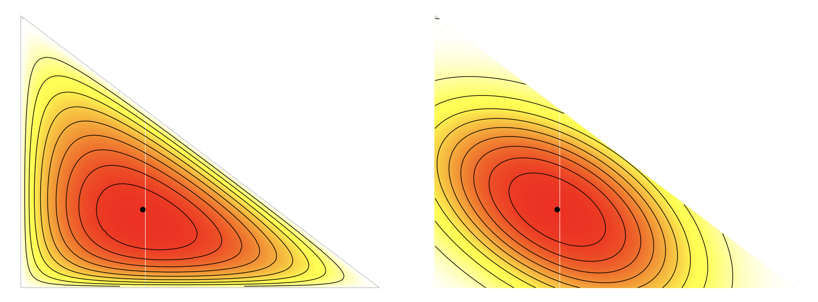
For $N=3$ this is easy to do because the simplex is a triangle. In the interactive demo (linked to the image above), select a distribution $p$ by clicking somewhere in the left triangle: the middle and right plots will then show a heat map of ‘distance’ to that point in cross-entropy and in the Euclidean metric respectively.
What we see is that the Euclidean metric does not know about the geometry of the space of distributions. Cross-entropy, on the other hand, grows to infinity as the second argument $q$ goes to the boundary. So, for example, if $p=(0.9,0.05,0.05)$ and $q=(1,0,0)$, then $p$ and $q$ are very close in the Euclidean metric, but infinitely far apart in cross-entropy.
(But note that this is not the case if $p$ and $q$ are reversed!! Cross-entropy is not symmetric, and is even linear in the first argument. You can see the effect of swapping direction of the distance measure using the menu below the middle plot.)
On the other hand, we do see that for distributions that stay away from the boundary — that is, for those with higher entropy — mean squared error is a surprisingly good approximation to cross-entropy, at least for $N=3$.
Of course, when we’re training neural networks, it’s precisely the low entropy, boundary distributions that matter. It’s the vertex points (one-hot distributions) that we use for training — in the vicinity of which cross-entropy is highly sensitive, while the Euclidean metric is blunt and unobservant.