What are geometric neural networks?
This is intended as working notes to get my head round some of the literature on geometric deep learning and Clifford algebra neural networks (NNs).
Contents:
1. Notation for NN layers
Recall that a NN layer is a function ${\bf x} \in {\mathbb R}^n \rightarrow {\bf y} \in {\mathbb R}^m$ of the form ${\bf \sigma} \circ W$ where $W$ is a $m \times n$ matrix and ${\bf \sigma} = (\sigma, \ldots , \sigma)$ is componentwise application of a nonlinear function $\sigma: {\mathbb R} \to {\mathbb R}$ (which maybe sigmoidal, or piecewise linear, or a step function, or something else).
A neural network is simply a composition of such layers.
Let $I$ be the index set {$1, \ldots , n $} for the units on the left (the components of ${\bf x}$) and $J$ the index set {$ 1, \ldots , m$} for the units on the right. It will be helpful to treat ${\bf x} , {\bf y}$ as functions $I \to {\mathbb R}$, $J \to {\mathbb R}$ respectively. To emphasise this, I’ll write ${\bf x} \in {\mathbb R}^I$ and ${\bf y} \in {\mathbb R}^J$.
We’ll first generalise $I,J$ to sets with more structure; then eventually we’ll generalise ${\mathbb R}$ to a bigger algebra.
2. Convolutional NNs
In the 2010s, the use of NNs for image processing was revolutionised by the introduction of convolutional NNs (CNNs). (See [1].)
In a CNN, we first take $I,J \subset {\mathbb Z}^2$. That is, NN units represent pixels in a 2D array. WLOG we can treat $I,J$ as equal to ${\mathbb Z}^2$ (but then constrain the support of the functions ${\bf x} , {\bf y}$). More precisely, we think of each of $I,J$ as the set ${\mathbb Z}^2$, acted on by the group ${\mathbb Z}^2$.
All or some of the layers of a CNN then have the form of a convolution: that is, the function $W{\bf x}: J \to {\mathbb R}$ is a convolution $K \star {\bf x}$ for some function (with finite support) $K: {\mathbb Z}^2 \to {\mathbb R}$.
In other words, the kernel $K$ is a filter which slides around the 2D pixel array $I$. Here’s a picture where $K$ has $2\times 2$ support:
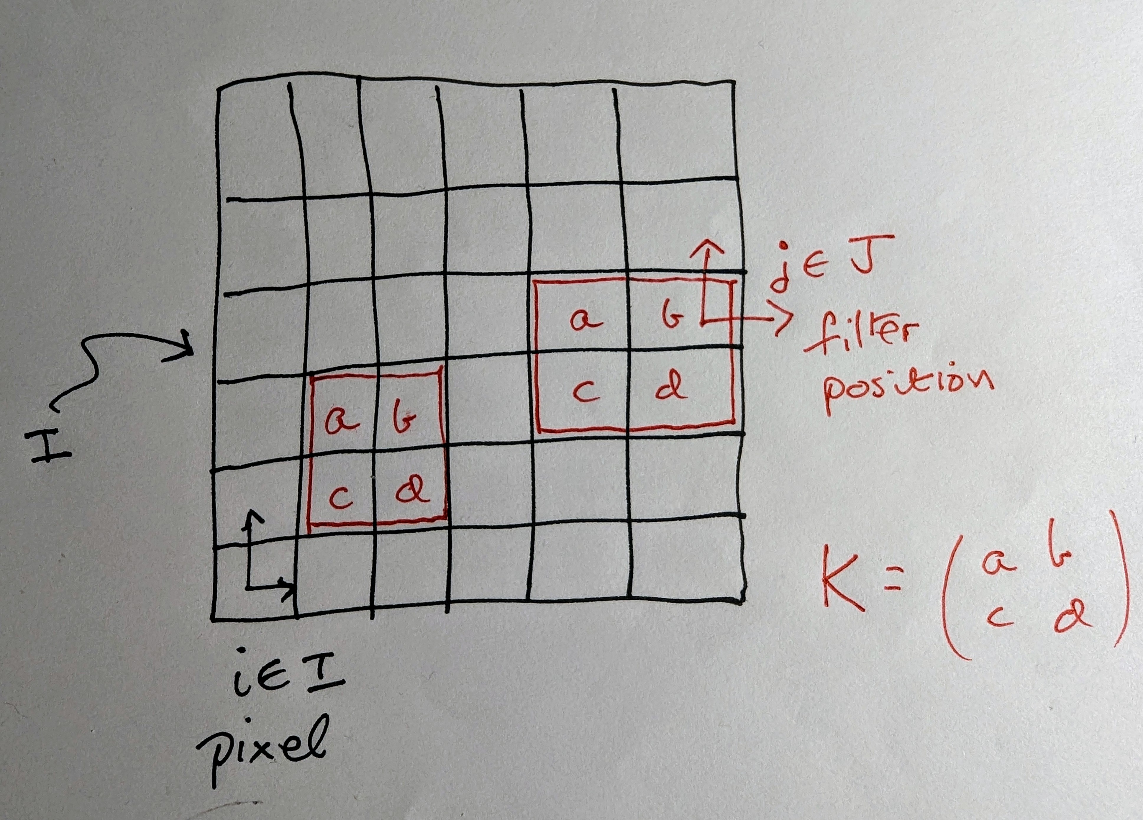
For a given pixel $i \in I$ and filter position $j \in J$, the linear coefficient $W_{ij}$ in the NN layer is simply the entry in $K$ over $i$ when the filter is at position $j$. (Exercise: write down a formula!)
What are the benefits of a convolutional layer?
- It’s efficient in model size: the matrix $W$ has $O(n)$ degrees of freedom instead of $O(n^2)$ (where $n = |I|$).
- It regularises across the image - reducing the likelihood of overfitting to treat the left-hand side of the image differently from the right-hand side, say.
- It is translation-equivariant. That is, as a function, the layer commutes with translation by ${\mathbb Z}^2$. If the image is shifted north-east a bit, the model won’t notice.
3. Group-equivariant CNNs
CNNs have a useful generalisation, first introduced in [2] (and probably elsewhere around that time). Suppose that a group $G$ acts on both $I,J$. For simplicity I’ll assume these actions are transitive - otherwise the arguments below are applied orbit-wise.
So we are generalising the case $G = {\mathbb Z}^2$ above. Just as in that case, we get induced actions on the functions ${\bf x}, {\bf y}$ by ${\bf x}^g (i) = {\bf x} (i^{g^{-1}})$ and similar for ${\bf y}$. We seek equivariance, meaning that these actions commute with $W$: \[ W {\bf x}^g = (W {\bf x})^g \qquad \hbox{for all $g \in G$.} \] In [2] it is shown that $W$ is equivariant in this sense if and only if it is convolutional: \[ W {\bf x} = K \star {\bf x} \in {\mathbb R}^J \qquad \hbox{for some $K \in {\mathbb R}^G$.} \] To be precise: fix some origins $i_0 \in I$ and $j_0 \in J$. Under the assumption of transitivity, any $i,j$ can be represented as $i = i_0^{g_i}$, $j = j_0^{g_j}$ for some $g_i, g_j \in G$. Then the convolution statement is equivalent to \[ W_{ij} = K(g_i^{-1} g_j). \]
Why does equivariance matter? If, as in the 2D image case, it is a natural requirement in the scenario we’re modelling, then it makes sense to build it into the mathemtical structure of the model. The alternative is that it is learned - imperfectly - from training data. Having equivariance (or invariance of the final output such as a classification of the image) built in directly represents an important saving in the data requirements for training.
4. Example: spherical CNNs
Here’s an example from [3]. Various 3D imaging applications need to model pixels on the 2-sphere - for example, from drone or satellite imagery.
In this case $I,J \subset S^2$ and $G$ is the 3D rotation group $SO(3)$. The matrix $W$ is a linear transformation of ${\bf x}: I = S^2 \to {\mathbb R}$ and is modelled as a convolution with a kernel $K : SO(3) \to {\mathbb R}$.
The group $SO(3)$ is 3-dimensional, with a coordinate chart given by Euler angles $\alpha,\beta,\gamma$. A kernel $K$ is specified to have bounded support in some window of $(\alpha,\beta,\gamma)$-space. The convolution is then expressed as an integral \[ (K \star {\bf x}) (R) = \int_{SO(3)} K(R Q^{-1}) {\bf x}(Q) dQ, \] whose computation requires some representation theory of $SO(3).$
Clifford algebras will offer a cleaner way to encode $SO(n)$ and $O(n)$-equivariance - and also with more tractable generalisation to $n > 3$.
Before coming to that, though, let’s remind ourselves that a NN model is to be learned from training data - how that is done, and how to incorporate convolutional layers in that process.
5. How convolutional kernels are learned from data
A neural network is a composite function $f: {\bf x} \to \cdots \to {\bf y}$ which seeks to model the conditional distribution $P(Y \mid X)$ for random variables $X,Y$. For example, $X$ may represent 2D pixel arrays and $Y$ the binary variable ‘image contains a cat’.
A training data set $D$ for $f$ consists of pairs $(x,y)$ drawn from the joint distribution of $X$ and $Y$. For each such pair we can evaluate $\hat{y} = f(x)$ and measure the distance $d(\hat{y}, y)$ (for a suitable metric $d$).
We can define an error function (usually called the loss function) \[ E_D(f) = \sum_{(x,y) \in D} d(\hat{y}, y). \] Training the model now means choosing the parameters of $f$ to minimise $E_D(f)$.
This minimisation takes place over linear coefficients in the $W$-matrices and kernels $K$ in the layers of the network. We assume the ‘architecture’ is fixed - that is, the number and size of layers, and the filter structure in the convolutional kernels.
We can assume WLOG that all layers are convolutional. That means we can treat the error as a function of the linear $K$ coefficients in all the layers, $E_D(K)$. This is a function over a big vector space, and we need to compute the derivative $\nabla_K(E_D)$.
Computing this derivative uses the chain rule. Let’s recall how this works.
Suppose, as an example, we want to differentiate the function \[ F(u,v) = u + v\sin(u+v). \] Here’s a picture of what we do:
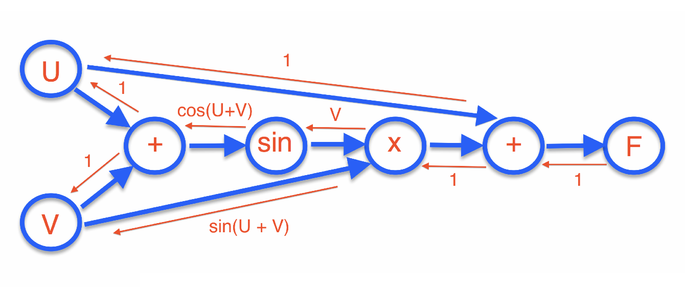
I’ve decomposed $F$ into a directed acyclic graph (DAG) of simple components. Evaluating the function involves a forward pass through this DAG.
The reverse (red) arrows are the computed derivatives of each arrow on its own. The chain rule for the end-to-end derivative can be written as: \[ \frac{\partial F}{\partial u} = \sum_{\hbox{paths $u \leftarrow F$}} \prod (\hbox{edges along the path}). \] (Exercise: check this for the example!)
The beauty of this formulation is that we don’t need to enumerate all the paths: we only need to pass messages back along the red edges, multiplying as we go and summing the incoming messages. The messages that arrive at the variables $u,v$ will then be the respective partial derivatives.
This formulation of the chain rule is called back-propagation. Let’s see how it works for the derivative $\nabla_K(E_D)$.
The DAG for the function $E_D(K)$ decomposes in the following way:
\[
\hbox{$K$ coeffs} \rightarrow \hbox{$W$ coeffs} \rightarrow \hbox{NN units} \rightarrow E_D.
\]
(Plus arrows among the NN units corresponding to network connections, not drawn.)
Back-propagation has only a simple derivative to compute along each edge in this graph.
6. Enter Clifford algebras
To motivate what comes next, let’s briefly compare two problems.
Problem 1: colour image classification.
Our input images now have three colour (RGB) channels, so we imagine a model with input \[ {\bf x} : I = {\mathbb Z}^2 \rightarrow {\mathbb R} \oplus {\mathbb R} \oplus{\mathbb R}. \] For this, an initial NN layer will be constructed by learning an independent kernel on each channel and summing the convolutions:
$$ K_{\rm red} \star {\bf x}_1 + K_{\rm blue} \star {\bf x}_2 + K_{\rm green} \star {\bf x}_3. $$
Problem 2: shallow water flow.
Here, the task is to predict fluid flow in the plane - that is to model velocity and pressure fields a few time steps in the future, given those fields now. So at each time step, input to the model looks like \[ {\bf x} : I = {\mathbb Z}^2 \rightarrow {\mathbb R} \oplus {\mathbb R}^2 \]
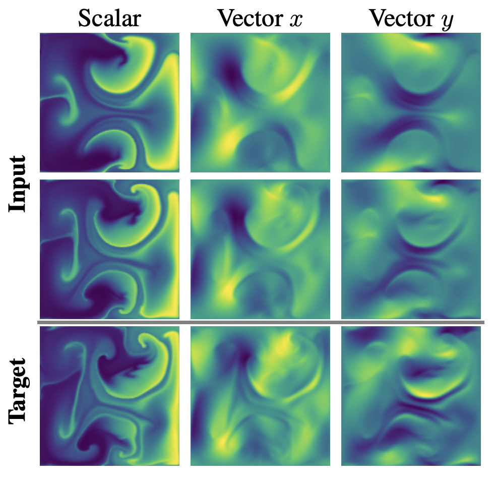
The standard approach would be to treat Problem 2 in the same way as Problem 1. However, this fails to exploit the geometric structure of the problem: two of the columns should be encoded not as independent scalars but as a single vector.
Mathematically, what this means is that we’d like to build in not just ${\mathbb Z}^2$-equivariance with respect to $I,J$, but $O(2)$-equivariance with respect to ${\mathbb R} \oplus {\mathbb R}^2$ (where $O(2)$ acts trivially on the first factor and as rotations/reflections on the second).
This can be achieved by treating ${\mathbb R} \oplus {\mathbb R}^2$ as contained in one of the Clifford algebras $Cl_{2,0}$ or $Cl_{0,2}$ (we can choose either). I’ll spell this out in just a moment, but the key thing to note is that as soon as \[ {\bf x} : I \rightarrow A \quad \hbox{and} \quad K : {\mathbb Z}^2 \rightarrow A \] (where $A$ is one of the two Clifford algebras) then convolution works exactly as before - all the formulae work fine over $A$ because we can add and multiply elements just as for ${\mathbb R}$.
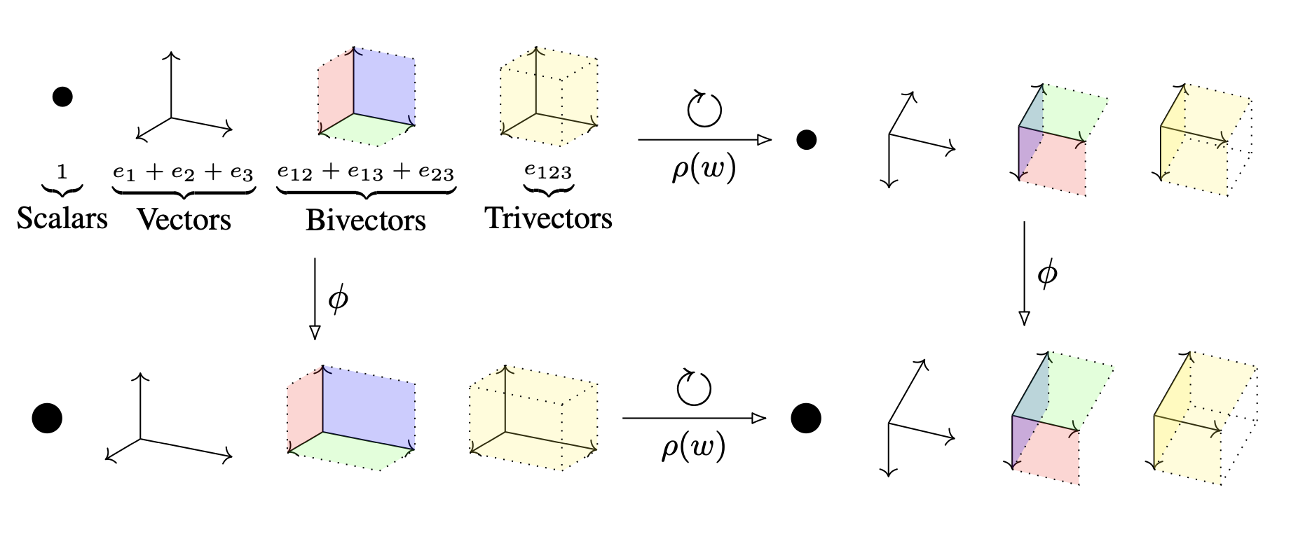
OK, so let’s spell this out. In both cases, $A$ has a basis $1, e_1, e_2, e_3 := e_1e_2$ where $e_1, e_2$ is a basis for the Euclidean ${\mathbb R}^2$ we’re interested in. By definition, \[ x^2 := \pm (x \cdot x) 1 \qquad \hbox{for $x \in {\mathbb R}^2 \subset A$.} \] The sign determines which of the two cases we’re in.
Case $A = Cl_{2,0}$ (called ‘Clifford Fourier’ in [6])
In this case $e_1^2 = e_2^2 = 1$ and it’s easy to check that $e_1 e_2 = - e_2 e_1$ and $e_3^2 = -1$. So we can write down an (algebra) isomorphism to real $2 \times 2$ matrices $Cl_{2,0} \cong {\mathbb R}(2)$
$$ 1 \mapsto \begin{pmatrix} 1 & 0 \\ 0 & 1 \end{pmatrix}, \quad e_1 \mapsto \begin{pmatrix} 0 & 1 \\ -1 & 0 \end{pmatrix}, $$$$ e_2 \mapsto \begin{pmatrix} 1 & 0 \\ 0 & -1 \end{pmatrix}, \quad e_3 \mapsto \begin{pmatrix} 0 & 1 \\ 1 & 0 \end{pmatrix}. $$
Exercise: show that for any ${ x}, { y} \in {\mathbb R}^2$, their product in
$Cl_{2,0}$ is
\[
{x} {y} = ({ x}\cdot { y}, 0,0, \det |{ x}\, { y}|) \in {\mathbb R}^4 \cong Cl_{2,0}.
\]
Case $A = Cl_{0,2}$ (called ‘rotational Clifford’ in [6])
In this case $e_1^2 = e_2^2 = -1$ but as in the previous case $e_1 e_2 = - e_2 e_1$ and $e_3^2 = -1$. So this time the algebra is isomorphic to the quarternions $Cl_{2,0} \cong {\mathbb H}$. If we want to we can represent the algebra as $2 \times 2$ complex matrices ${\mathbb H} \subset {\mathbb C}(2)$. Then the basis elements map to the Pauli matrices
$$ 1 \mapsto \begin{pmatrix} 1 & 0 \\ 0 & 1 \end{pmatrix}, \quad e_1 \mapsto \begin{pmatrix} 0 & i \\ i & 0 \end{pmatrix}, $$$$ e_2 \mapsto \begin{pmatrix} 0 & 1 \\ -1 & 0 \end{pmatrix}, \quad e_3 \mapsto \begin{pmatrix} -i & 0 \\ 0 & i \end{pmatrix} $$
where $i = \sqrt{-1}$.
Whether we choose to learn rotational or Fourier Clifford kernels is a design choice, as are other aspects of the NN architecture. For either choice, the kernels are learnt (by back-propagation) and deployed in exactly the same way as for layers defined purely over ${\mathbb R}$ - but now the $O(2)$-geometric structure is built in.
For 3D problems, where we want a model to respect $O(3)$ geometry, the story is similar. The Clifford algebra (for choice of signature, or choice of sign on the Euclidean inner product) is 8-dimensional over ${\mathbb R}$, with basis illustrated in the picture at the top of these notes. It’s a fine graphic - but for my money less useful than a clear representation of the algebra in terms of matrices over ${\mathbb R}$, ${\mathbb C}$ or ${\mathbb H}$.
So (exercise!) - we can find isomorphisms \[ Cl_{3,0} \cong {\mathbb H} \oplus {\mathbb H} \] (where multiplication is componentwise) and \[ Cl_{0,3} \cong {\mathbb C}(2) \] (all $2 \times 2$ complex matrices). Again, one can learn (from data) and work with convolutional kernels taking values in either of these algebras.
And so on for higher dimensions.
7. A short zoo of applications
The following list summarises some of the experiments and applications described in the references. It’s not complete, but I’ve separated the symmetries of the index space $I$ from those of the values taken by ${\bf x} : I \to V$.
| Application | Index space $I$ | Value space $V$ | Reference |
|---|---|---|---|
| Image classification | ${\mathbb R}^2$ up to translation | ${\mathbb R}$ | [1] |
| Spherical images | ${S}^2$ up to $SO(3)$ | ${\mathbb R}$ | [3] |
| Signed volume of a polyhedron | $n$ indices | ${\mathbb R}^3$ up to $SO(3)$ | [5] |
| Convex hull of points | $n$ indices up to $S_n$ | ${\mathbb R}^5$ up to $O(5)$ | [5] |
| O(5)-invariant regression | {0,1} | ${\mathbb R}^5$ up to $O(5)$ | [5] |
| $n$-body system | $n$ indices | ${\mathbb R}^3$ up to $E(3)$ | [5] |
| Navier-Stokes PDE | ${\mathbb R}^2$ up to translation | ${\mathbb R} \oplus {\mathbb R}^2$ up to $SO(2)$ | [6] |
| Maxwell's PDE | ${\mathbb R}^3$ up to translation | ${\mathbb R}^3 \oplus {\mathbb R}^3$ up to $SO(3)$ | [6] |
References
- Ian Goodfellow, Yoshua Bengio, Aaron Courville, Deep Learning, MIT Press (2016)
- Taco Cohen, Max Welling, Group equivariant convolutional networks, arXiv.1602.07576 (2016)
- Taco S. Cohen, Mario Geiger, Jonas Koehler, Max Welling, Spherical CNNs, arXiv.1801.10130 (2018)
- Michael M. Bronstein, Joan Bruna, Taco Cohen, Petar Veličković, Geometric Deep Learning: Grids, Groups, Graphs, Geodesics and Gauges, arXiv.2104.13478 (2021)
- David Ruhe, Johannes Brandstetter, Patrick Forré, Clifford group equivariant neural networks, arXiv.2305.11141 (2023) (code here)
- Johannes Brandstetter, Rianne van den Berg, Max Welling, Jayesh K. Gupta, Clifford neural layers for PDE modelling, arXiv.2209.04934 (2023) (code here)
- David Ruhe, Jayesh K. Gupta, Steven de Keninck, Max Welling, Johannes Brandstetter, Geometric Clifford algebra networks, arXiv.2302.06594 (2023)