Navigating the PLOS ONE topic tree

PLOS ONE is a respected multidisciplinary journal publishing research from
over two hundred subject areas across science, engineering, medicine, and the related social sciences and humanities.
But exactly how many subject areas?
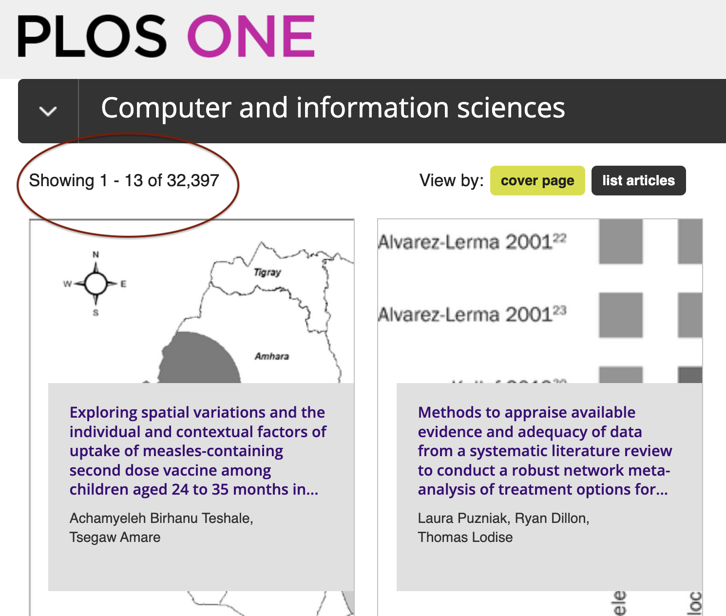
At the top level (as shown in the screenshot above), these subject areas fall under eleven headings from Biology and life sciences to Social sciences. For each of these headings – such as Computer and information sciences below - we are told the number of articles (in this case 32,397) and can browse further subheadings:

This post is about a short exercise to scan the entire tree of PLOS ONE topics, asking:
- how does one extract and represent this tree?
- are the article counts per topic consistent e.g. in the sense that each count is the sum of the counts at the leaves of the corresponding subtree?
Visually, the result of the analysis is plots such as the following (the topic trees of some of the top-level headings):
1. Crawling
The starting task was to crawl the PLOS ONE pages. To do this, we initialise a data frame with a single row (I’ll use Python-like pseudocode throughout - most of this exercise was actually done in R):
topic_tree_df.add_row('node' = 1,
                      'parent' = 1,
                      'topic' = "",
                      'parent_topic' = "",
                      'count' = None)
… and then add tree nodes to the data frame via the following breadth-first search:
browse_url = "https://journals.plos.org/plosone/browse/"
index = 1

while index <= nrow(topic_tree_df):
  this_topic = topic_tree_df[index, 'topic']
  url = browse_url + this_topic
  topic_tree_df[index, 'count'] = find_count(url)    # read HTML
  next_batch = find_children(url)                    # read HTML
  for child in next_batch:
    topic_tree_df.add_row('node' = row.index
                          'parent' = index,
                          'topic' = child,
                          'parent_topic' = this_topic
                          'count' = None
                          )
  index += 1
In this code, the functions find_count() and find_children() parse the HTML of the currently visited topic page and extract the count and subtopics respectively. (For this I use the package rvest in R.)
2. Counting
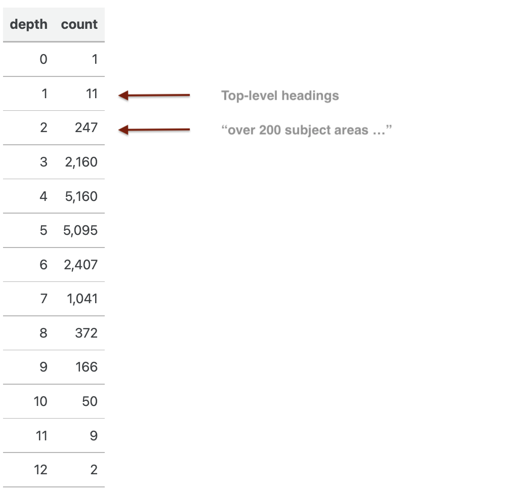
The code generates a data frame with (as of 9 Feb 2022) a total of 16,721 rows (topics). From this data frame we can read off any tree statistics - for example the node count by depth in the tree:
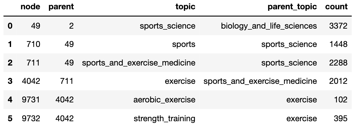
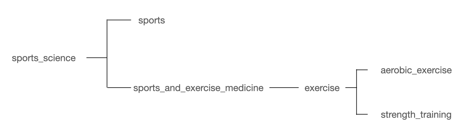
To illustrate the data frame, the following slice is the part of the tree below node 49, sports_science. (This is an example of a clade: a subtree that exactly consists of one node and all its descendants:)
The first thing to note is that the article counts (as read off from the PLOS ONE topic pages) are not in any sense consistent! (That was question 2 at the top of this post.)
At each node, we can read off an excess count, which is the difference between the advertised article count and the sum of the counts at child nodes. This excess is usually positive: for example, at the topic exercise the excess is 1,515 - the number of articles that presumably do not fall under the subtopics of aerobic_exercise or strength_training. This is to be expected if the topic tree grows over time with new subtopics being added to the PLOS thesaurus. On the other hand, the excess count is often negative. For example, the count at sports_science is actually less than the counts at its two subtopics sports and sports_and_exercise_medicine. At some point, the parent node has stopped counting!
(It turns out that the excess count has a large negative value at all of the 11 top-level topics – which are therefore underestimating the number of articles they cover.)
3. Drawing
Finally, a word about tree formats and visualisation. The circular plots shown above could have been made using a package like R phylotools. In fact, I took a shortcut and used the very convenient Interactive Tree Of Life (iTOL) site.
In either case, a more compact data format is needed than the data frame shown above. A popular format that I used is the Newick format. The idea of Newick format is that the tree is represented by a string with the recursive form
\[ \nu({\rm tree}) = (\nu({\rm child}_1),\ldots,\nu({\rm child}_k))\nu({\rm root}) \]
and where $\nu({\rm single\ node})$ is any convenient string representing that node, e.g. the topic name. Converting from the data frame shown above to Newick format is then achieved with a simple recursive function:
def newickR(tree_df, j):
    out = ""
    if exist children(j):
        out = "("                           # open bracket
        for i in children(tree_df, j):      # insert commas-separated child strings
            out += newickR(tree_df, i) + ','
        if out[-1] == ',':                  # remove final comma
            out = out[:-1]
        out += ')'                          # close bracket
    out += tree_df[j,'topic']               # append parent string
    return out
Applied to the little sports_science data frame this outputs:
> newickR(tree_df, 0)
  '(sports,((aerobic_exercise,strength_training)exercise)sports_and_exercise_medicine)sports_science'