Watching a neural network learn a Markov chain
Modern language models derive their power from big data and big compute – but also, ultimately, from the Unreasonable Effectiveness of Recurrent Neural Networks described by Andrej Karpathy (and many others) a decade or so ago. This post is more low-brow than Karpathy’s — I wanted to explore a little bit how RNNs perform on some carefully controlled toy data: specifically on sequences generated from Markov chains.
What does it mean to model a sequence? It means two things:
- Given a new sequence generated by the same process, can we predict at each time step the next sequence item?
- Does the ‘model’ give simplying insights into this underlying process?
Suppose, for example, that the sequence is drawn from an ‘alphabet’ of $N$ distinct symbols, and that the process generating the sequence is Markov — in other words, each item depends only on its predecessor. In that case, problem 1 is completely solved in $O(N^2)$ storage by just collecting enough data and observing conditional frequencies. This does nothing to address problem 2, however. On the other hand, fitting an $n$-state hidden Markov model (HMM) reduces the storage to $O(nN)$. So it improves the solution to problem 1 — but it also answers problem 2 if we can interpret what the ‘hidden states’ mean.
However, most sequences generated by processes of interest are not 1-st order Markov. If the process is Markov of order $k$, then the storage requirement for the naive solution is $O(Nk)$, which rapidly becomes intractable. This is where RNNs come in. At least, they appear to perform well on problem 1. What about problem 2? Can we extract any understanding from them?
Here’s an example. It’s a stretch of ASCII sequence (from a source which I’ll reveal in a moment):
ikkviiviiekotkiwiwiieeiiioikttooiotkkeiiokkttkkiwvvwtkikweiwvwikkkiokkwookkkkoiikiieiiiwoivveiioikokiivikoiooookkikkvwveikookkutktktvvwktkkwwkiwiwikkuktkkoiwkkkkotewiikkiukkvwwktkkokkieeiiwiookkiiiiot
Let’s see what we can learn by fitting a recurrent network (of Long Short-Term Memory (LSTM) units). Since the sequence only exhibits a small alphabet consisting of {e,i,k,o,t,u,v,w}, I’m not going to expend a huge model on it, so I choose an RNN architecture consisting of just one hidden layer with 2 units.
Having trained this small network, let’s observe the output of those two inner units — as points in the plane ${\mathbb R}^2$ — as we pass the sequence through it:
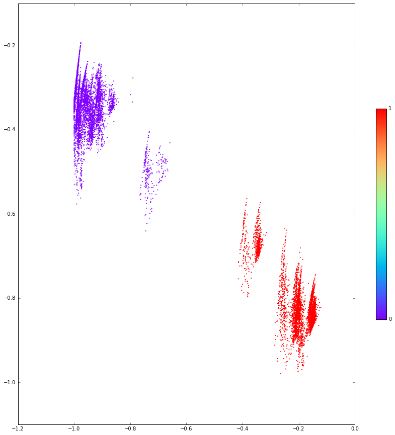
What are the colours? Well, I now need to reveal that the sequence was generated from a 2-state hidden Markov model with states (where the coefficients are shorthand for probabilities of the state outputting each character):
\[ 0.496 {\tt k} + 0.302 {\tt o} + 0.157 {\tt t} + 0.045 {\tt u} \]
\[ 0.106 {\tt e} + 0.562 {\tt i} + 0.117 {\tt v} + 0.215 {\tt w} \]
together with some randomly chosen $2\times 2$ transition matrix for moving between the states. I’ve coloured the plot above by the HMM state. What we see is that this internal structure is effectively discovered by the RNN. (So it gives us some help with question 2 above. I’ll come to question 1 in a moment.)
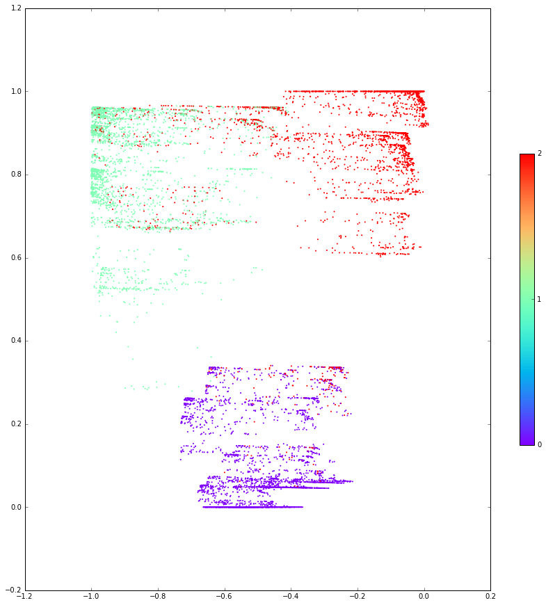
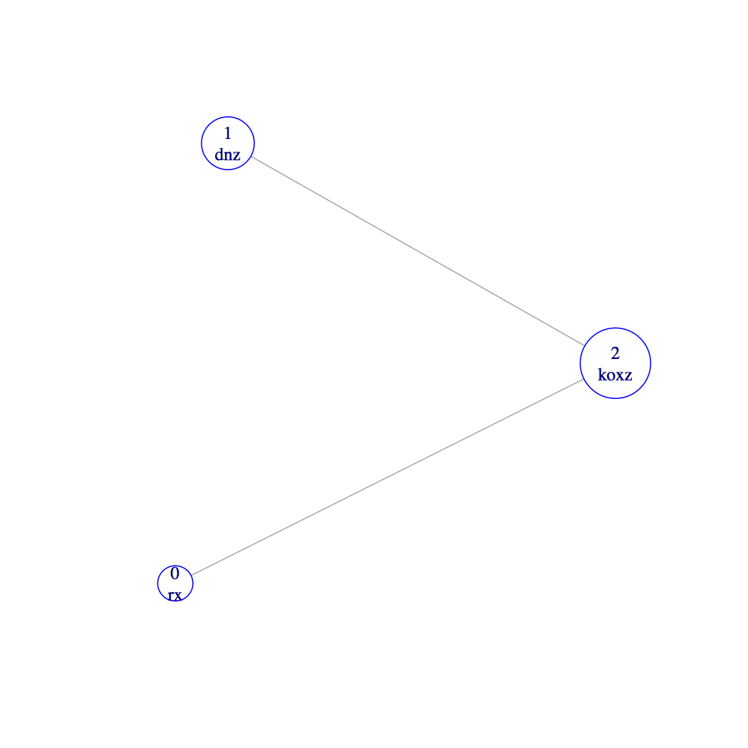
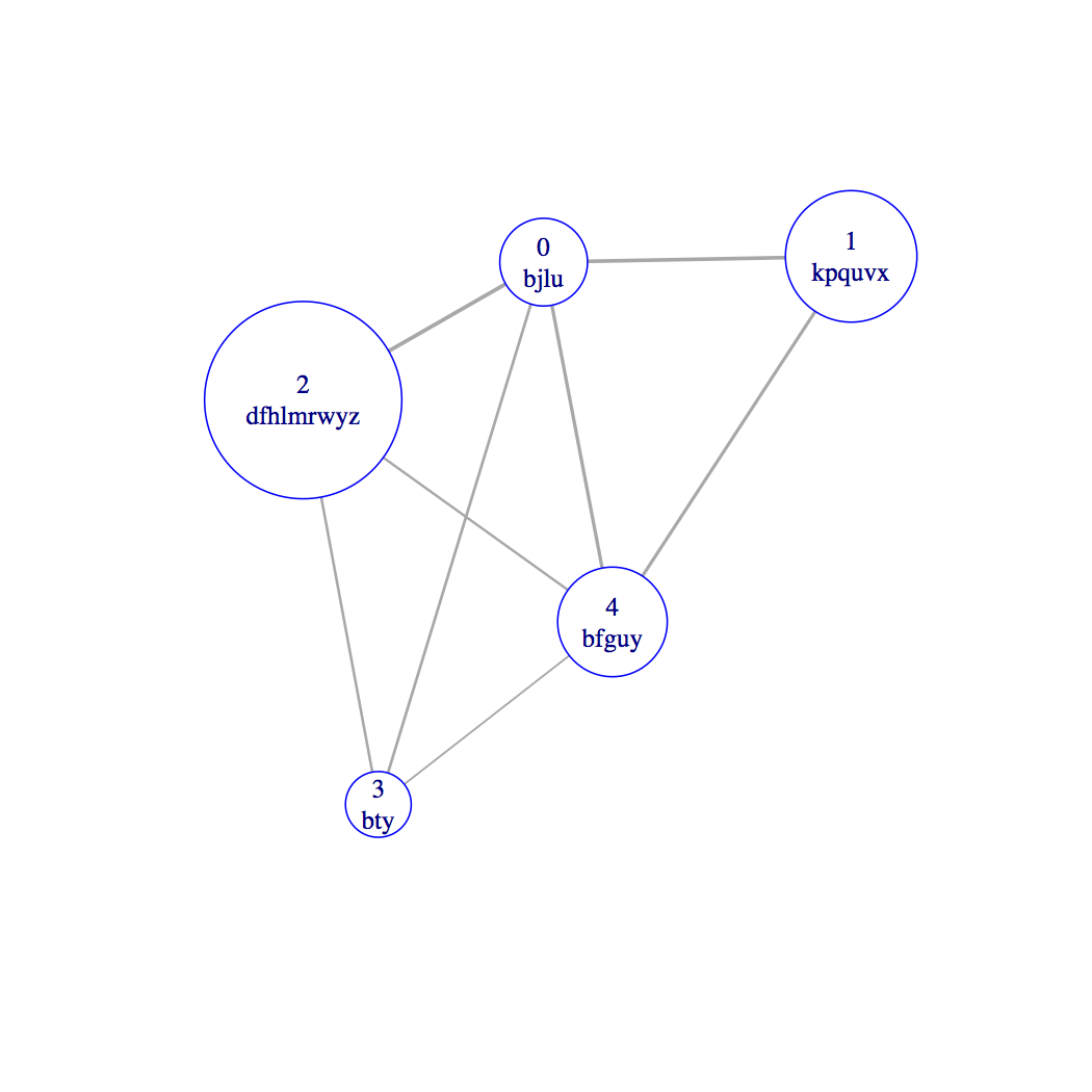
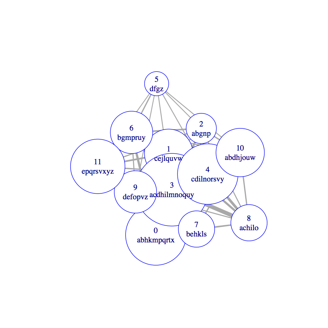
This example was very easy because the HMM states are ‘far apart’: they output completely disjoint sets of characters. Let’s look at some other examples. The first does the same as above, but for data generated from a 3-state HMM with closer (overlapping) output distributions. The graph on the right represents the HMM states, with edges representing overlap (actually, closeness of the output distributions using their total variation):
xrrxzzkkzzrxkrzzkkkkzrzoxzkoxrzzzkkzkoznzznznrxxrkkxxrxrrrkrznzxzznzrnnxxxxrrzkkznkkzknznnkzkkokkzzkrrkxknzzoozzzzzzzzzzzoknzzdrroznzzzzznznzznnrxokkxrrozkxrzzkkkrrrxxokkoozkokzzxookozzndzzokzkkxkzxrz
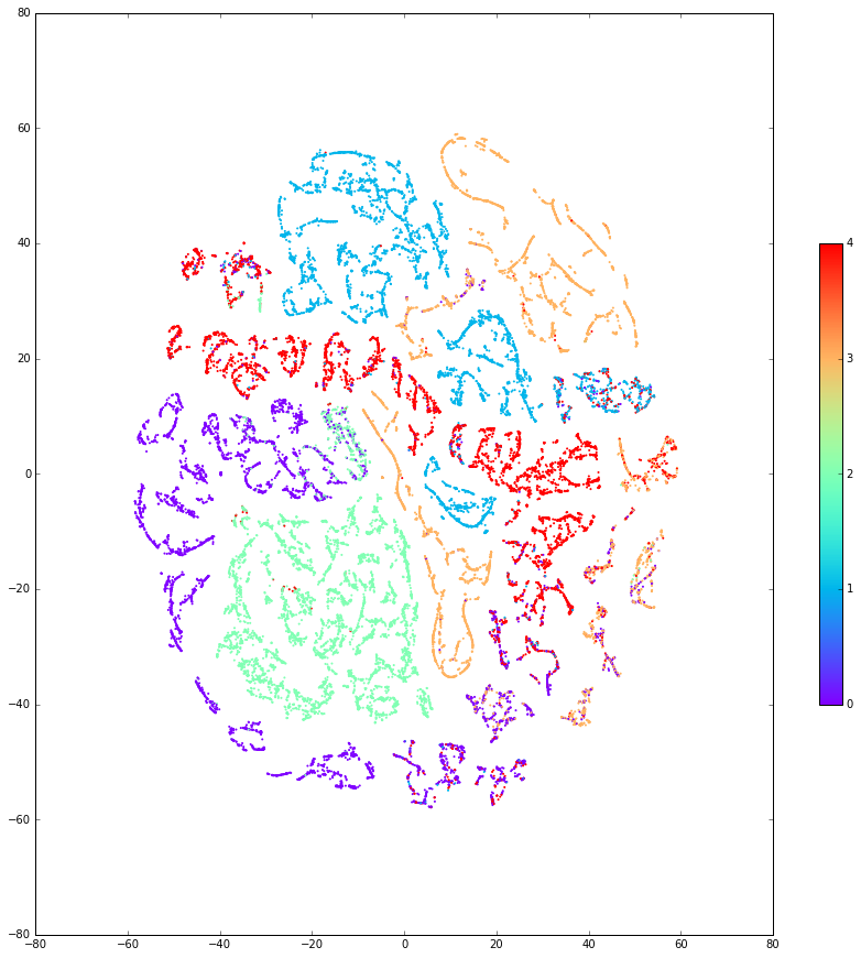
Next are two examples using 3 units in the RNN layer, so that now the sequences are represented in ${\mathbb R}^3$. They both use data generated from a 5-state HMM, but with different state configurations:
becbcbyooooeceyyjyywccbbbnenennneybooyyywbooobnbyobooobeewyoooywyjwjjywoeeooooooooonbbybbeennnbbccbwyybooennoooooooooooooooooooooooyjwjbbbbbeoobbybeeebyybenegjywyywygenyyybbceennennnnnwjyybbboooecccbb
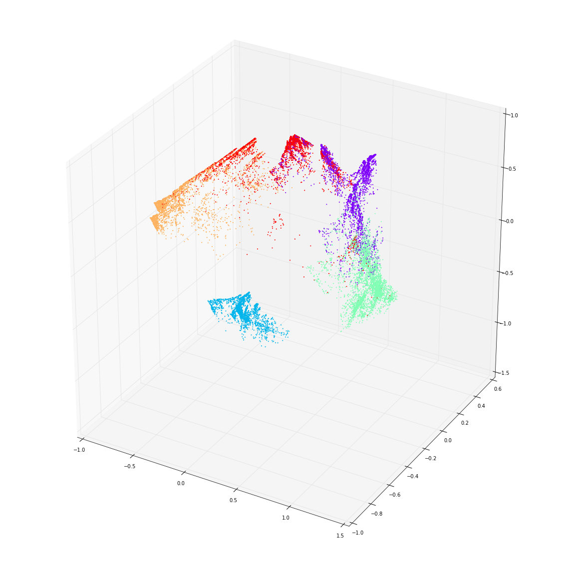
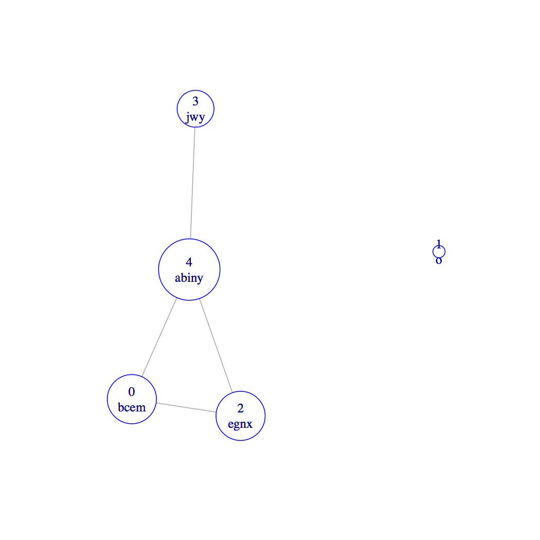
Here, we see that ‘confusion’ between HMM states is well represented in the RNN. The least confused HMM state is state 1, which is uniquely distinguished by outputting only ‘o’, and is coloured blue in the 3-dimensional plot. The most confused state is 4 (red). But remember that the RNN is not trying to distinguish the HMM states — it knows nothing about them — it is simply representing the observed structure of the output sequence. Of course, this structure reflects both the hidden states and their output distributions.
kqxvklljguguuuybywfrywrmkvbygglyuuguggggubjljwrwpulljuulrwwrrwugugguuummlppkzlrguupkpkpbytyupkxubuugtbyywhwuvxwrpvupppvybwlwrdpubgyuyxuuuugupxpuxuprwzfbjujljullugukwdzwrtbbbbtbybbbbtuugwfwffuguugbujbb
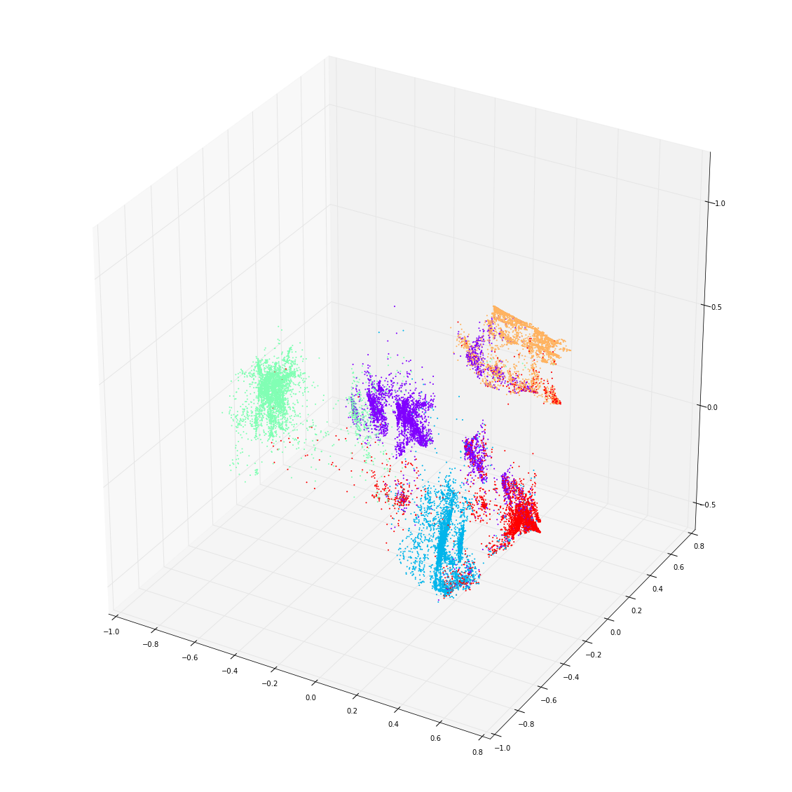
This last example has the most confusion among HMM states, and that is reflected in the 3-dimensional plot. Nevertheless, if we do a dimensional reduction to the plane using $t$-SNE for this example, we see that the separation is in fact still pretty good:
How well do these RNN models answer problem 1 above? How well do they predict sequence outputs? Let’s focus on the last example.
First note that the way we don’t want to assess the predictive power of the model is to measure symbol error rate. That way, when we are dealing with inherently high entropy distributions, madness lies. In other words, in our situation each character is generated from a distribution which may be close to uniform, with multiple characters equally likely. Guessing the right one correctly may not tell us very much about the model — what we really need to know is that the model is giving us the right probability distribution.
Since we have a God’s eye view of the data (it is generated from a Markov chain that we specified!) we know exactly what the right probability distribution is. That is, we know the (HMM) state transition matrix $P$ and the emission matrix $F$ (whose rows are the character distributions conditional on the HMM state). As we observe a sequence generated by the HMM, we can compute the ‘alpha’ vector as we go (which gives the joint probability of a given HMM state with the characters observed so far). Multiplying the alpha (row) vector on the right by the product $PF$ gives the distribution of the next character conditional on the sequence so far observed — exactly what we want.
The RNN knows nothing about the HMM states, but is also outputting, as a softmax, its estimate of the same conditional distribution at each time step. The correct measure of its performance, therefore, as is how close this softmax is to the HMM-derived distribution.
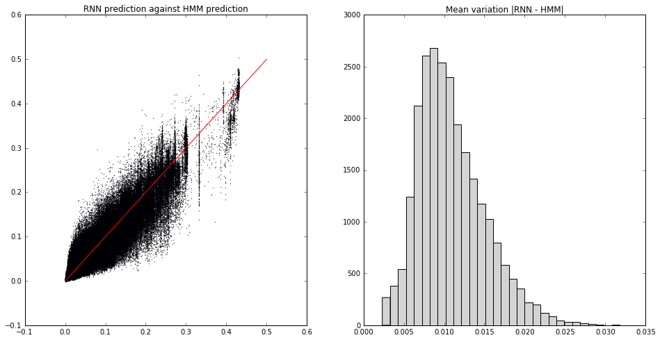
Here’s the comparison for the last example above. On the left I’ve plotted, for all possible next characters at all time steps in a test sequence a few thousand long, the predicted RNN (softmax) probability against the actual (HMM) probability. The histogram on the right shows the (mean per time-step) absolute value of the difference:
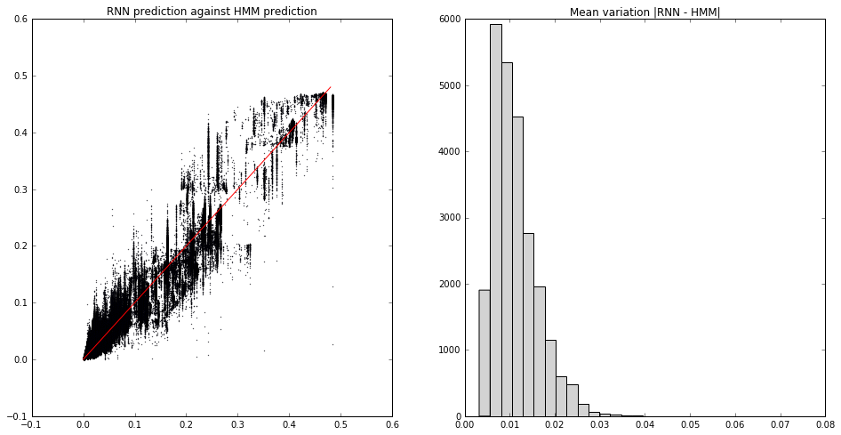
What we see is that the median discrepancy is around 1%. Not bad! Just for good measure, here’s a slightly hard example, with 12 well-mixed HMM states and using a 16-unit RNN (so the coloured plot is a $t$-SNE reduction from ${\mathbb R}^{16}$):
cjydlrmppyygmmmyvprcchcmchauncanpngehshssllshhdolliaicaobdnnnabylroloddpgrbgprpyrpysyxzffefvzvzzewhsabgppyggehlpppyyalolnlddlvebnpbanbnfzebxvvfvbanbnnnoldlnnpnpabwbooupgppubvvfzvvviiaihhspphovvvveshlh
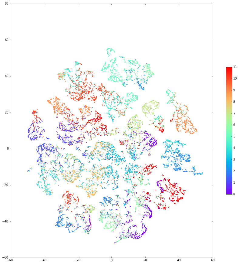
We get a comparable performance, with median discrepancy around 1%.
We can (and should!) also ask how these predicted probabilities (by HMM or by RNN) compare with what we actually observe. (This is after all a test we can always apply, not just for toy Markov-generated data.)
In the plot below I’ve divided the interval $[0,1]$ into 20 bins. For each bin I’ve counted the proportion of character predictions with (HMM or RNN) probability in this range that actually happen. In other words, we’d like to see, if the model is well calibrated, that around 20% of prediction at 0.2 actually happen, and so on. I’ve plotted these proportions (blue for HMM, red for RNN), and the closer the plot to the diagonal, the better calibrated the model:
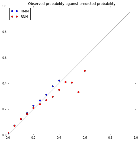
(Incidentally, being just above the diagonal is actually correct, because the observed proportion has been plotted against the bottom of the corresponding bin range.)
This shows where the RNN performance is weaker. But up to this point I haven’t said anything about the details of training the RNN. In particular, it’s common to use dropout to prevent overfitting, and the calibration plot above was actually the result of training the RNN without any dropout. Since this calibration is a good measure of the RNN performance, we should compare with an RNN trained with dropout (20% on the dense connections between layers):
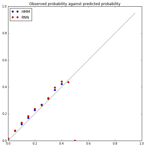
So now the RNN is pretty well spot on.
What’s needed now is a mathematical analysis to explain the observations above, to tell us how they will scale, how they will extend to high-order dependencies, and how the RNN performance will depend on architecture and training parameters.